Bulk RNA-seq Analysis
Overview
The goal of this analysis is to identify differentially expressed genes (DEG) between responders and non-responders in the HVP01 study using the bulk RNA-seq data.
From whole blood transcriptome profiling, we have bulk RNA-seq data for 15 subjects over 5 time points (visit day 0,1,3,7,14). The studied Hepatitis B Vaccine (drug: ENGERIX®-B) consists of three doses. After each dose, response to the vaccination is determined by the anti-HBs antibody level above 10 mIU/mL.
In this report, we focus on the response after dose 2 (with 13 responders and two non-responders). At a single time point, we perform a naive t-test. To include multiple time points, we also perform the parametric PBtest, which takes into account the repeated measurement data structure.
This report is organized in the following sections.
- Sample table: vaccine response and other meta data for each sample.
- Single time point analysis: t-test for response after dose 2 with Day 7 data only.
- Multiple time points analysis: parametric PBtest for response after dose 2 with all time points.
Load useful packages.
library(genefilter)
library(PBtest)
In the following analyses, significance level is set at 5%. Benjamini-Hochberg multiple testing correction will be applied.
alpha <- 0.05Sample table
Earlier, we read in “HVP_sampleTable_response_May18.csv” to ctab, which contains the dose response and other clinical information for each sample in the expression matrix.
kable(ctab) %>%
  kable_styling(bootstrap_options = c("hover")) %>%
scroll_box(width = "100%", height = "300px")| Sample_name | Subject_id | Visit_day | Responder_dose1 | Responder_dose2 | Age | Age_Group | Sex |
|---|---|---|---|---|---|---|---|
| GR01_V3 | GR01 | 0 | Yes | Yes | 57 | young | F |
| GR01_V4 | GR01 | 1 | Yes | Yes | 57 | young | F |
| GR01_V5 | GR01 | 3 | Yes | Yes | 57 | young | F |
| GR01_V6 | GR01 | 7 | Yes | Yes | 57 | young | F |
| GR01_V7 | GR01 | 14 | Yes | Yes | 57 | young | F |
| GR02_V3 | GR02 | 0 | No | Yes | 60 | old | F |
| GR02_V4 | GR02 | 1 | No | Yes | 60 | old | F |
| GR02_V5 | GR02 | 3 | No | Yes | 60 | old | F |
| GR02_V6 | GR02 | 7 | No | Yes | 60 | old | F |
| GR02_V7 | GR02 | 14 | No | Yes | 60 | old | F |
| GR03_V3 | GR03 | 0 | No | Yes | 52 | young | F |
| GR03_V4 | GR03 | 1 | No | Yes | 52 | young | F |
| GR03_V5 | GR03 | 3 | No | Yes | 52 | young | F |
| GR03_V6 | GR03 | 7 | No | Yes | 52 | young | F |
| GR03_V7 | GR03 | 14 | No | Yes | 52 | young | F |
| GR04_V3 | GR04 | 0 | Yes | Yes | 73 | old | F |
| GR04_V4 | GR04 | 1 | Yes | Yes | 73 | old | F |
| GR04_V5 | GR04 | 3 | Yes | Yes | 73 | old | F |
| GR04_V6 | GR04 | 7 | Yes | Yes | 73 | old | F |
| GR04_V7 | GR04 | 14 | Yes | Yes | 73 | old | F |
| GR05_V3 | GR05 | 0 | No | Yes | 69 | old | M |
| GR05_V4 | GR05 | 1 | No | Yes | 69 | old | M |
| GR05_V5 | GR05 | 3 | No | Yes | 69 | old | M |
| GR05_V6 | GR05 | 7 | No | Yes | 69 | old | M |
| GR05_V7 | GR05 | 14 | No | Yes | 69 | old | M |
| GR06_V3 | GR06 | 0 | No | Yes | 53 | young | M |
| GR06_V4 | GR06 | 1 | No | Yes | 53 | young | M |
| GR06_V5 | GR06 | 3 | No | Yes | 53 | young | M |
| GR06_V6 | GR06 | 7 | No | Yes | 53 | young | M |
| GR06_V7 | GR06 | 14 | No | Yes | 53 | young | M |
| GR07_V3 | GR07 | 0 | No | Yes | 44 | young | M |
| GR07_V4 | GR07 | 1 | No | Yes | 44 | young | M |
| GR07_V5 | GR07 | 3 | No | Yes | 44 | young | M |
| GR07_V6 | GR07 | 7 | No | Yes | 44 | young | M |
| GR07_V7 | GR07 | 14 | No | Yes | 44 | young | M |
| GR09_V3 | GR09 | 0 | No | Yes | 51 | young | F |
| GR09_V4 | GR09 | 1 | No | Yes | 51 | young | F |
| GR09_V5 | GR09 | 3 | No | Yes | 51 | young | F |
| GR09_V6 | GR09 | 7 | No | Yes | 51 | young | F |
| GR09_V7 | GR09 | 14 | No | Yes | 51 | young | F |
| GR10_V3 | GR10 | 0 | No | Yes | 55 | young | F |
| GR10_V4 | GR10 | 1 | No | Yes | 55 | young | F |
| GR10_V5 | GR10 | 3 | No | Yes | 55 | young | F |
| GR10_V6 | GR10 | 7 | No | Yes | 55 | young | F |
| GR10_V7 | GR10 | 14 | No | Yes | 55 | young | F |
| GR11_V3 | GR11 | 0 | No | Yes | 50 | young | F |
| GR11_V4 | GR11 | 1 | No | Yes | 50 | young | F |
| GR11_V5 | GR11 | 3 | No | Yes | 50 | young | F |
| GR11_V6 | GR11 | 7 | No | Yes | 50 | young | F |
| GR11_V7 | GR11 | 14 | No | Yes | 50 | young | F |
| GR13_V3 | GR13 | 0 | No | Yes | 46 | young | F |
| GR13_V4 | GR13 | 1 | No | Yes | 46 | young | F |
| GR13_V5 | GR13 | 3 | No | Yes | 46 | young | F |
| GR13_V6 | GR13 | 7 | No | Yes | 46 | young | F |
| GR13_V7 | GR13 | 14 | No | Yes | 46 | young | F |
| GR15_V3 | GR15 | 0 | No | Yes | 44 | young | F |
| GR15_V4 | GR15 | 1 | No | Yes | 44 | young | F |
| GR15_V5 | GR15 | 3 | No | Yes | 44 | young | F |
| GR15_V6 | GR15 | 7 | No | Yes | 44 | young | F |
| GR15_V7 | GR15 | 14 | No | Yes | 44 | young | F |
| GR17_V3 | GR17 | 0 | No | No | 63 | old | F |
| GR17_V4 | GR17 | 1 | No | No | 63 | old | F |
| GR17_V5 | GR17 | 3 | No | No | 63 | old | F |
| GR17_V6 | GR17 | 7 | No | No | 63 | old | F |
| GR17_V7 | GR17 | 14 | No | No | 63 | old | F |
| GR18_V3 | GR18 | 0 | No | No | 72 | old | M |
| GR18_V4 | GR18 | 1 | No | No | 72 | old | M |
| GR18_V5 | GR18 | 3 | No | No | 72 | old | M |
| GR18_V6 | GR18 | 7 | No | No | 72 | old | M |
| GR18_V7 | GR18 | 14 | No | No | 72 | old | M |
| GR19_V3 | GR19 | 0 | No | Yes | 62 | old | M |
| GR19_V4 | GR19 | 1 | No | Yes | 62 | old | M |
| GR19_V5 | GR19 | 3 | No | Yes | 62 | old | M |
| GR19_V6 | GR19 | 7 | No | Yes | 62 | old | M |
| GR19_V7 | GR19 | 14 | No | Yes | 62 | old | M |
Single time point analysis
In vaccine studies, it is common to look at the Day 7 post-vacctine data given the time lag between vaccination and immune activation. At the single time point, we can simply use the t-test to compare between the responders and non-responders.
T-test for response after dose 2 with Day 7 data
## subset Day 7 column data
ctab.D7 <- ctab %>% filter(Visit_day==7)

## t-test
out.t.D7 <- rowttests(dat.filt10.symbol[,ctab.D7$Sample_name], as.factor(ctab.D7$Responder_dose2))
padj.t.D7 <- p.adjust(out.t.D7$p.value, method="BH")
names(padj.t.D7) <- rownames(out.t.D7)
(sig.gene.D7 <- names(which(padj.t.D7<alpha))) #1 DEG
## [1] "WSB2"head(sort(padj.t.D7)) #top genes## WSB2 TMEM201 MYBL2 SYT17 ZNF142 AAK1
## 0.03943521 0.07863648 0.42500969 0.56207867 0.56207867 0.56207867There is only 1 DEG identified using sinlge time point at Day 7. The following plot shows that this gene is under-regulated in the responders.
## plot
plot(dat.filt10.symbol[sig.gene.D7,ctab.D7$Sample_name],
     col=as.factor(ctab.D7$Responder_dose2), pch=19,
     xlab="Subject", ylab="Day 7 expression level",
     main=paste0(sig.gene.D7, ", p-value = ", round(padj.t.D7[sig.gene.D7],3)))
legend("topleft", c("Non-responder","Responder"), col=1:2, pch=19)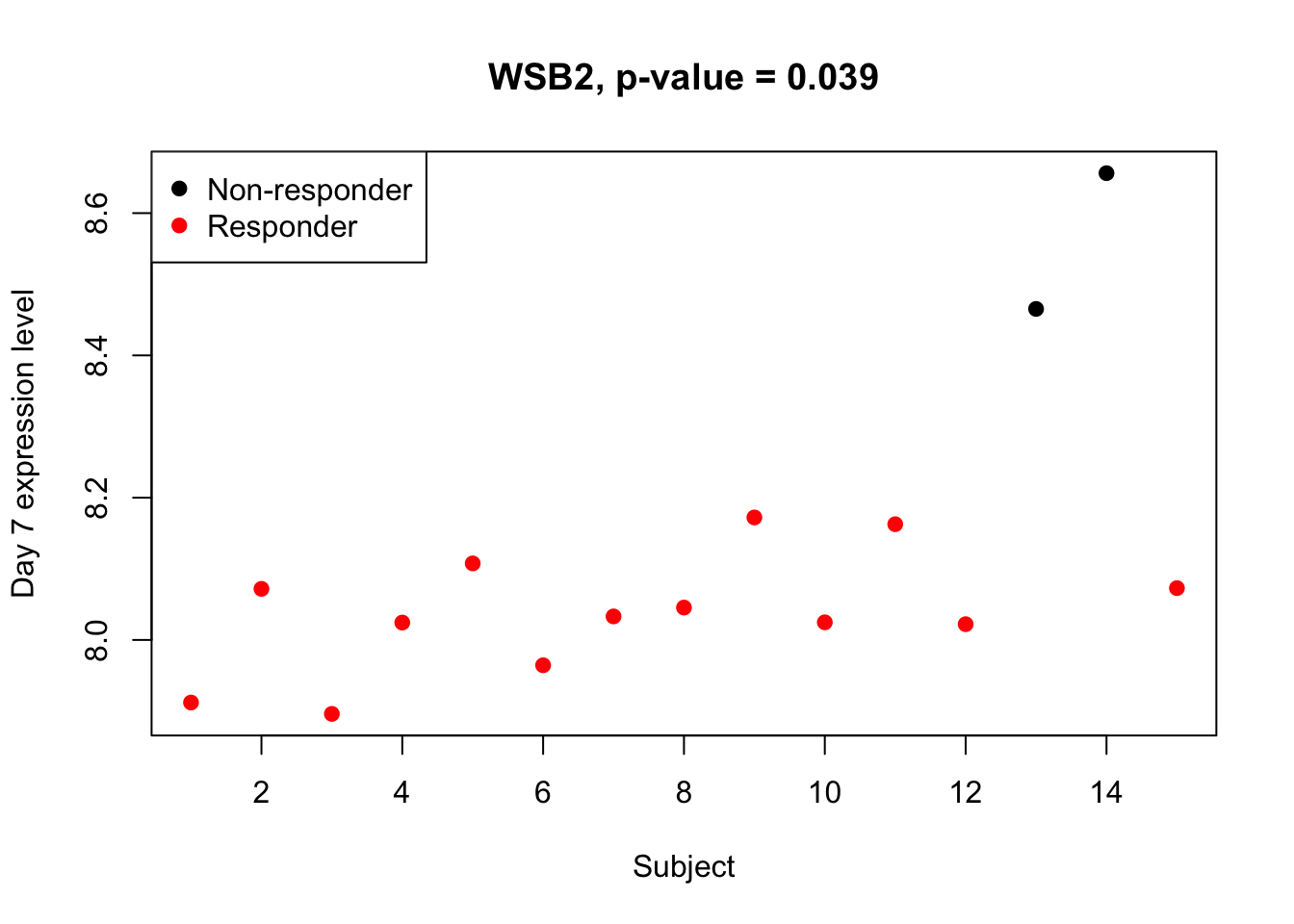
Multiple time points analysis
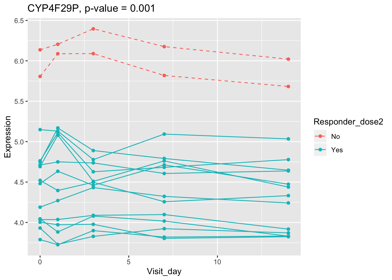
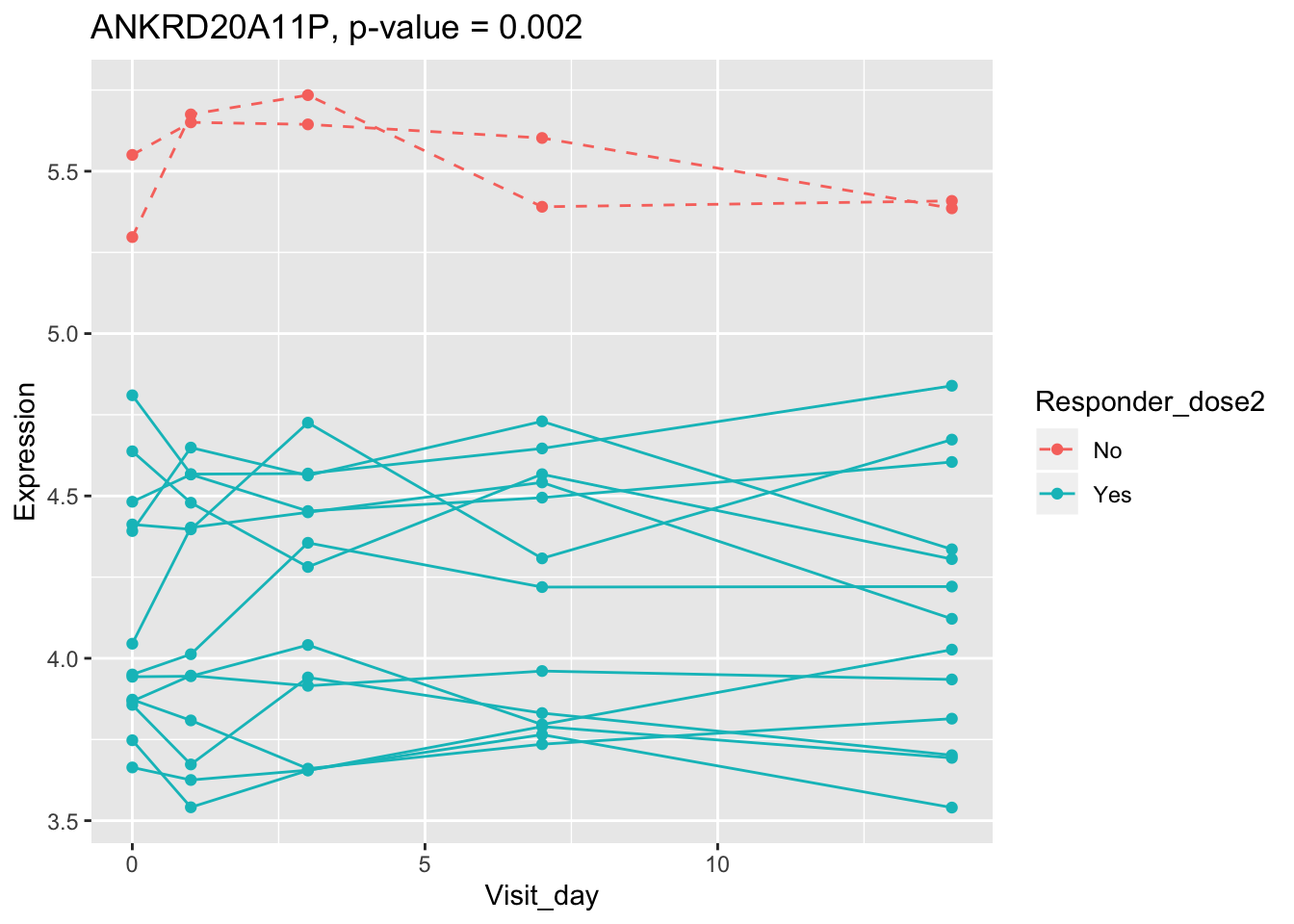
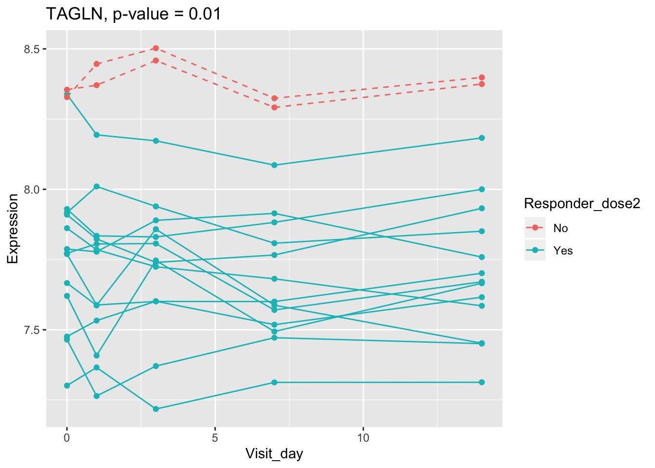
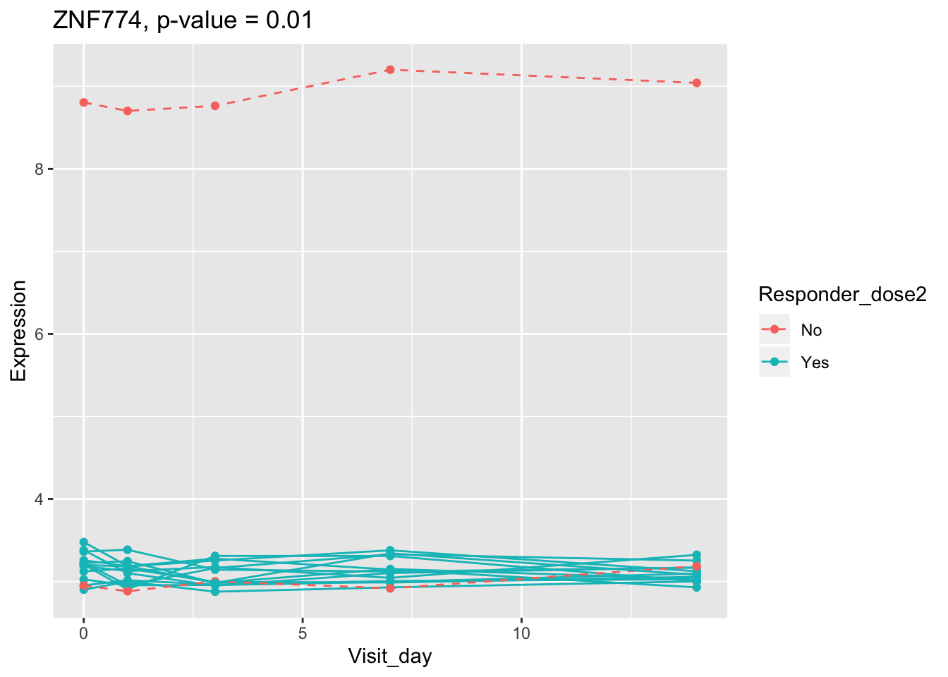
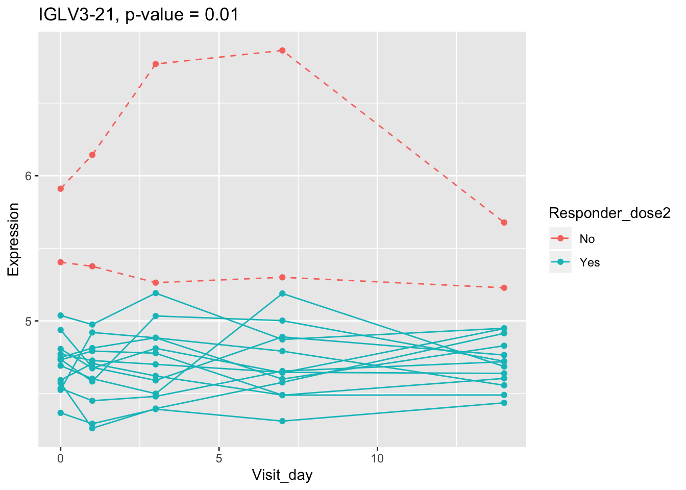
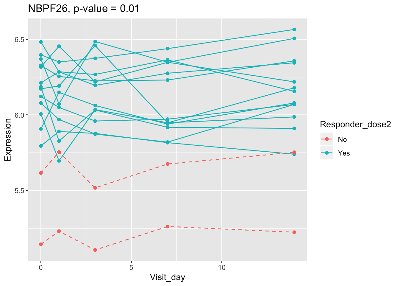
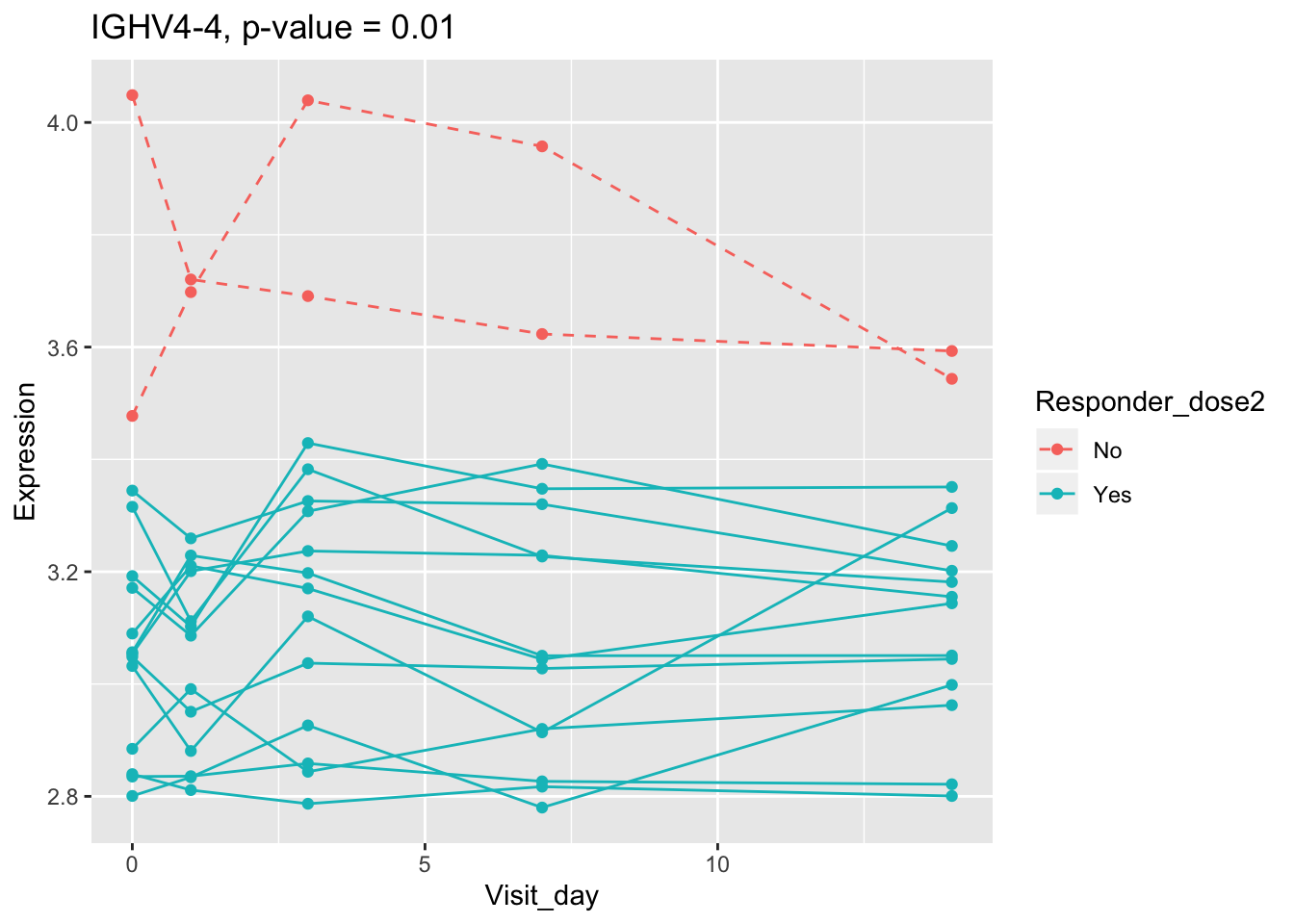
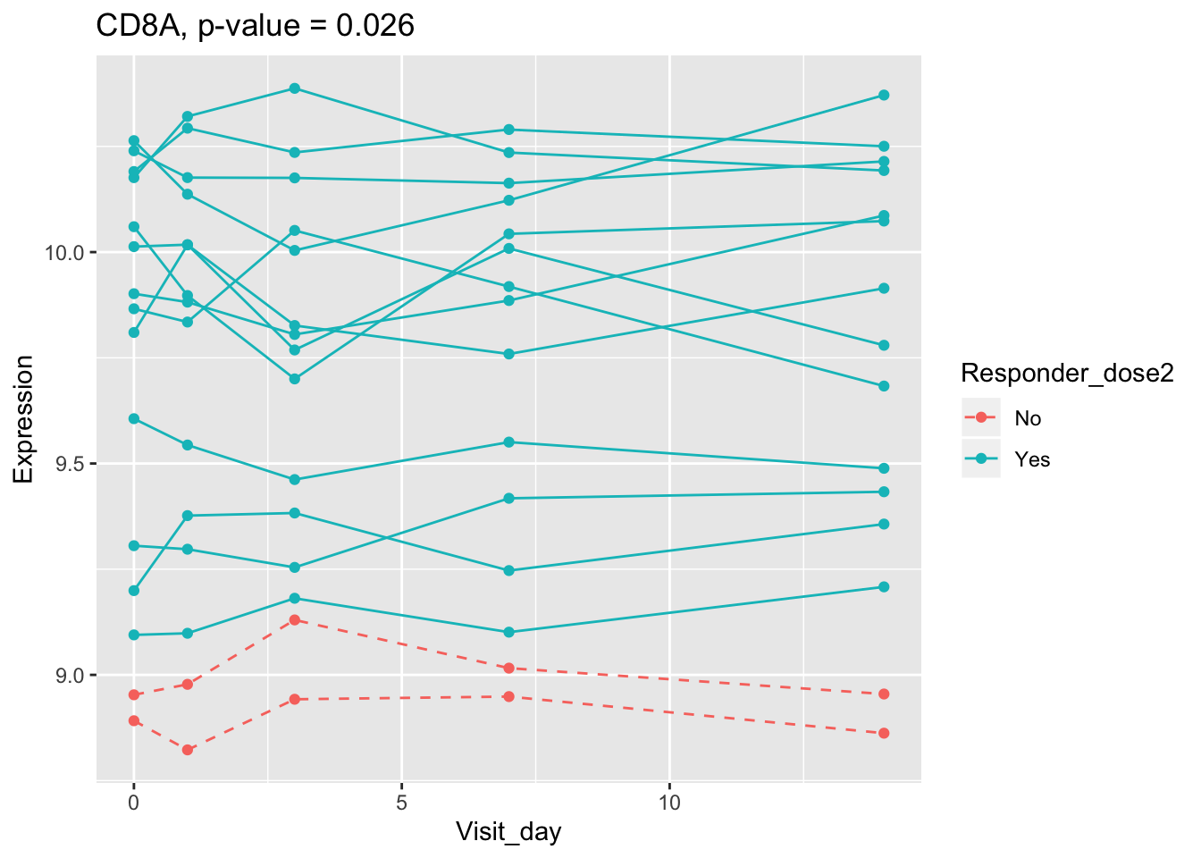
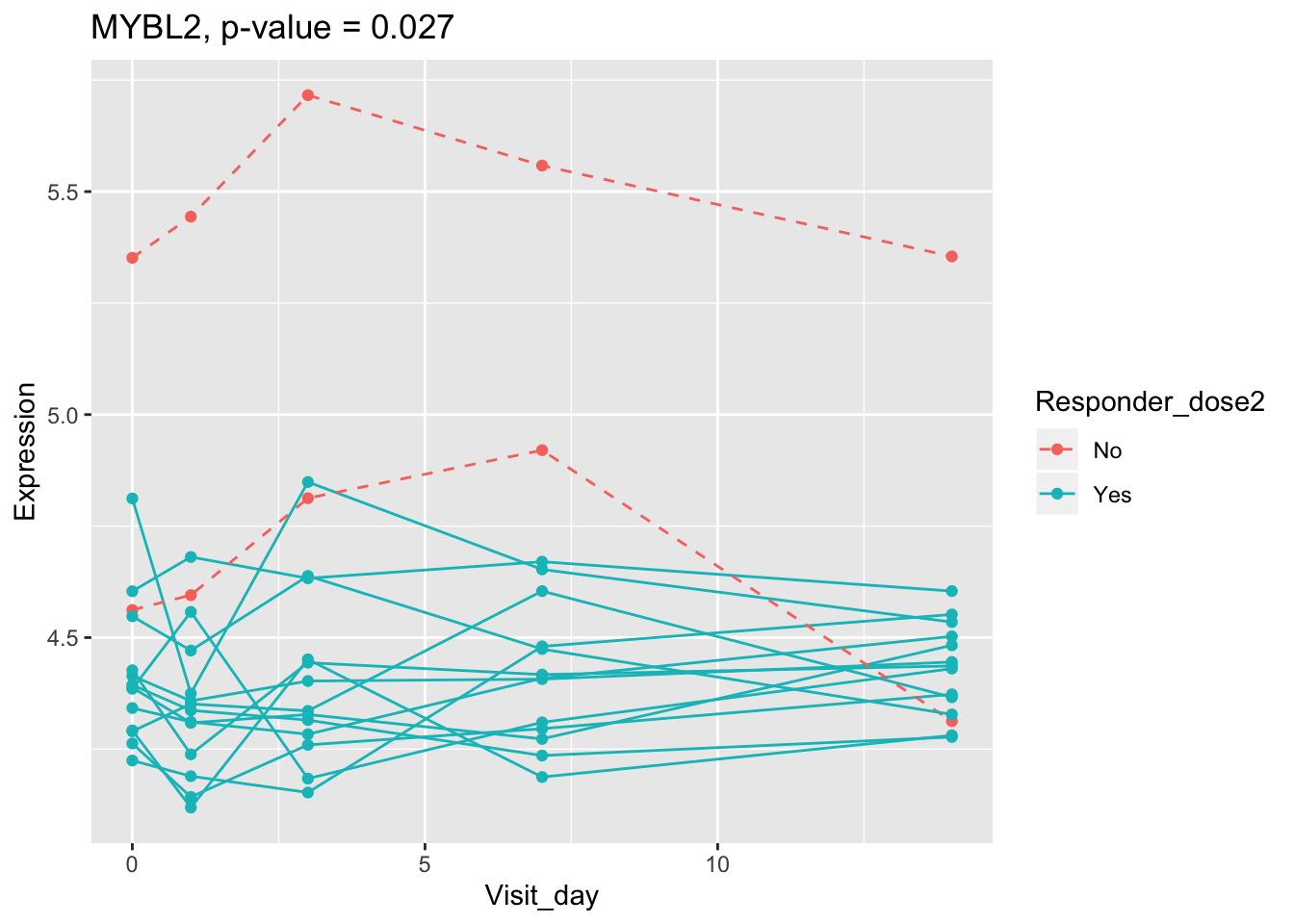
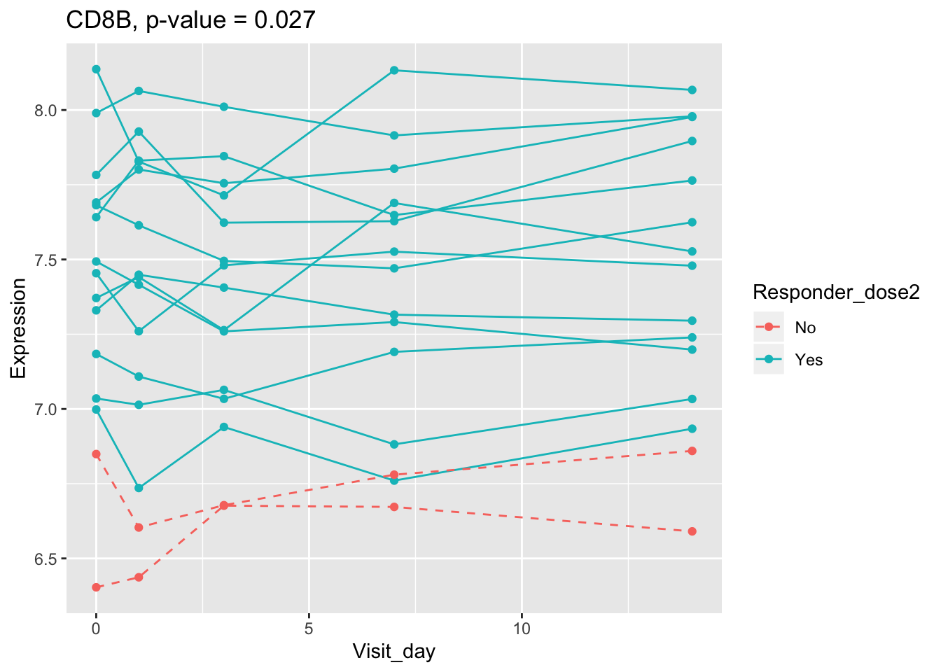
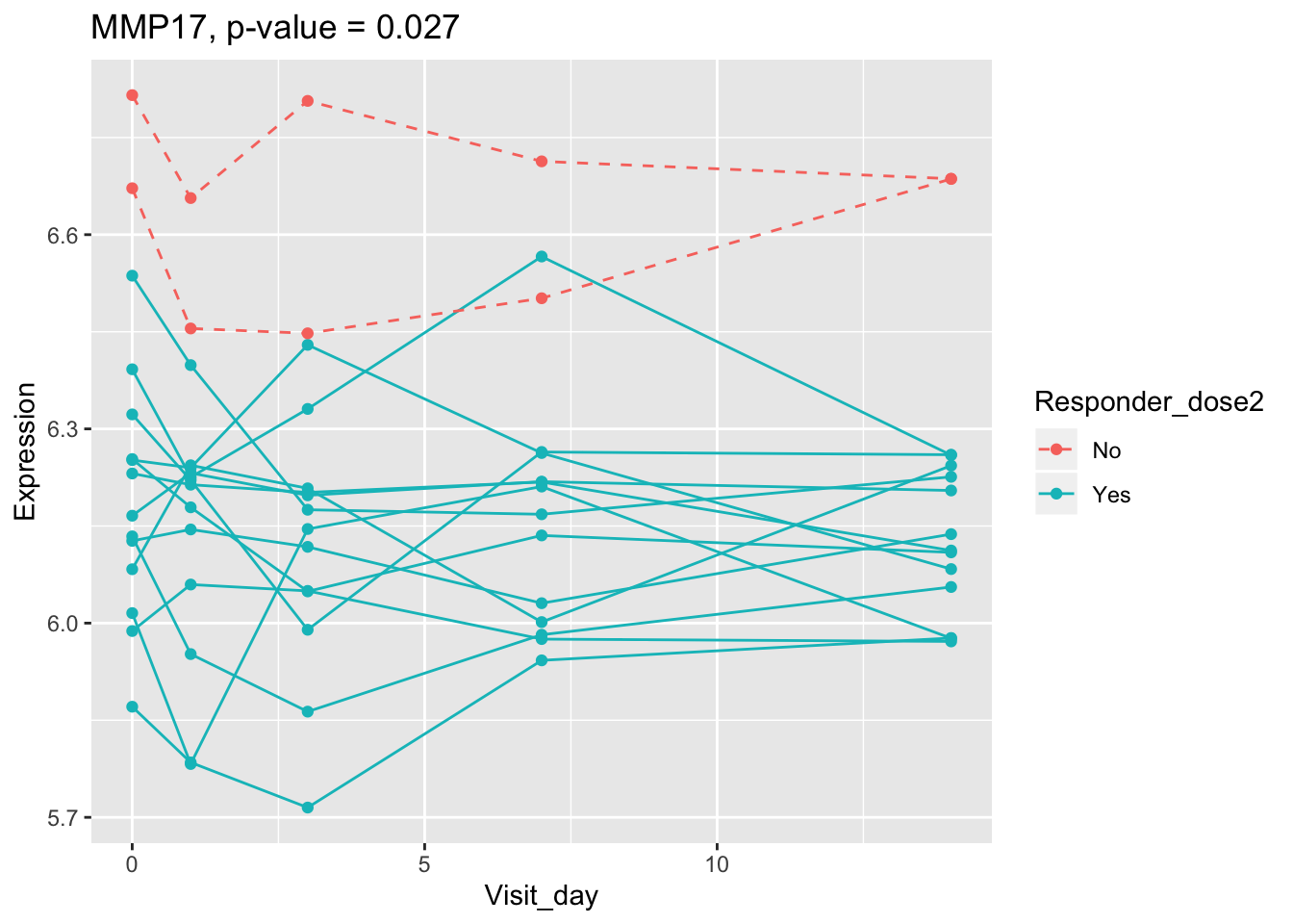
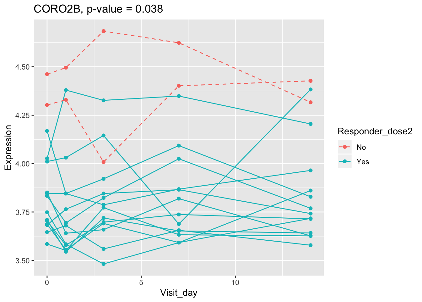
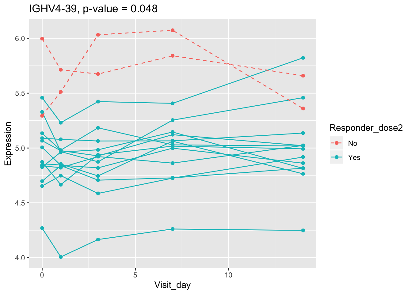
Immune response is a dynamic procedure. Using just one time point limits the scope of our analysis. With PBtest, a highly efficient hypothesis testing method for regression-type tests with correlated observations and heterogeneous variance structure, we are able to include all time points available in the study. It reveals more DEGs between the responders and non-responders.
PBtest for response after does 2 with all time points
## PBtest
out.PBtest <- PBtest(YY=t(dat.filt10.symbol),
                     xx=as.factor(ctab$Responder_dose2),
                     id=ctab$Subject_id)
padj.PBtest <- p.adjust(out.PBtest$p.value, method="BH")
names(padj.PBtest) <- names(out.PBtest$p.value)
padj.PBtest.sorted <- sort(padj.PBtest)
(sig.gene.PBtest <- names(padj.PBtest.sorted)[padj.PBtest.sorted<alpha]) #14 DEGs
## [1] "CYP4F29P" "ANKRD20A11P" "TAGLN" "ZNF774" "IGLV3-21"
## [6] "NBPF26" "IGHV4-4" "CD8A" "TCL1A" "MYBL2"
## [11] "CD8B" "MMP17" "CORO2B" "IGHV4-39"padj.PBtest.sorted[1:30] #top genes## CYP4F29P ANKRD20A11P TAGLN ZNF774 IGLV3-21
## 0.001209757 0.001523306 0.009972987 0.009972987 0.009972987
## NBPF26 IGHV4-4 CD8A TCL1A MYBL2
## 0.009972987 0.009972987 0.025889548 0.027076586 0.027315378
## CD8B MMP17 CORO2B IGHV4-39 LARGE1
## 0.027315378 0.027315378 0.037506093 0.047982663 0.058518654
## IGHD THEMIS JUP IGHV3-21 CTD-3064M3.3
## 0.058518654 0.061576042 0.061576042 0.061576042 0.061576042
## HLA-DMB SHTN1 IGHV1-3 RP11-164H13.1 CDKN1C
## 0.063839415 0.065953526 0.087418335 0.087638782 0.096983455
## IGLV6-57 HDHD3 CPVL EOMES TCL6
## 0.107899649 0.114981091 0.122971924 0.124335118 0.124335118Using all time points, 14 DEGs are identified using PBtest. The following plots show the expression levels of those DEGs across time in responders and non-responders.
## plot
for(gene in sig.gene.PBtest){
  x <- dat.filt10.symbol[gene,]
  df.x <- ctab %>% mutate(Expression=x)
  g <- ggplot(data=df.x, aes(x=Visit_day, y=Expression, group=Subject_id, colour=Responder_dose2)) +
    geom_line(aes(linetype=Responder_dose2)) + geom_point() +
    scale_linetype_manual(values=c("dashed", "solid")) +
    ggtitle(paste0(gene, ", p-value = ", round(padj.PBtest[gene],3)))
  plot(g)
}