Data Prep
Overview
The goal of this data preprocessing procedure is to filter and transform the RNA-seq count data of the HVP01 Immunity to Hepatitis B Vaccine study, so that the filtered and transformed data follows approaximately a constinuous normal distribution, which can then be fitted by advanced statistical models, such as the linear mixed-effect regression model, for differential analysis and deconvolution analysis.
Our general strategy of preprocessing RNA-seq count data follows three steps:
- Filter low count and low variance genes.
- Choose a data transformation that transforms the count data to some normally distributed data. For RNA-seq, it specifically means to
- transform discrete data to continuous data, and
- stabilize the mean-variance relationship, i.e. mitigate overdispersion.
- Plot the filtered and transformed data distribution, and adjust the choices from previous two steps if needed.
This report is organized in the following sections.
- A brief recap of DESeq2 data transformations. One naive transformation and two DESeq2 transformation techniques.
- Naive log2-tranformation
- Variance stabilizing transformations (VST)
- Regularized logarithm (rlog)
- Original count data. Apply the above three transformations on the original count data. One caveat is that the original count data are slightly filtered by the data provider. However, the data plots show excessive low count genes.
- Gene filtering. Filter out low count and low variance genes, and apply the three transformations on the filtered data.
- Final preprocessed data. Pick up the best data transformation and save the final data.
Load useful packages.
library(DESeq2)
library(vsn) #for menaSdPlot
A brief recap of DESeq2 data transformations
Briefly, the DESeq2 R package provides two alternative approaches that offer more theoretical justification than the naive log2-transformation on RNA-seq count data. One makes use of the concept of variance stabilizing transformations (VST) (Tibshirani 1988; Huber et al. 2003; Anders and Huber 2010), and the other is the regularized logarithm (rlog), which incorporates a prior on the sample differences (Love, Huber, and Anders 2014). Both transformations produce transformed data on the log2 scale which has been normalized with respect to library size or other normalization factors.
For more information, please see DESeq2 Bioconductor page.
Original count data
We obtain the original count data from our data provider in the file “HVP_countMatrix_noGlobin_May18.csv”, which contains filtered counts (genes with <10 counts across 5 samples are removed). These have also had the globin genes removed.
mycount <- read.csv("../HVP_countMatrix_noGlobin_May18.csv", row.names = 1)
ctab <- read.csv("../HVP_sampleTable_response_May18.csv")
dim(mycount)
## [1] 15026 75The original count data has 15026 genes and 75 samples. Next, we build the DESeq2 data object for our count data.
## build dds object from count data
dds <- DESeqDataSetFromMatrix(countData = mycount,
                              colData = ctab,
                              design = ~ 1) #for the design formula, check out the "blind=TRUE" option in the transformation step
log2-transformation on original count data
## log2-transformation
ntd <- normTransform(dds)
mat0 <- assay(ntd)
hist(rowMeans(mat0), breaks=50)
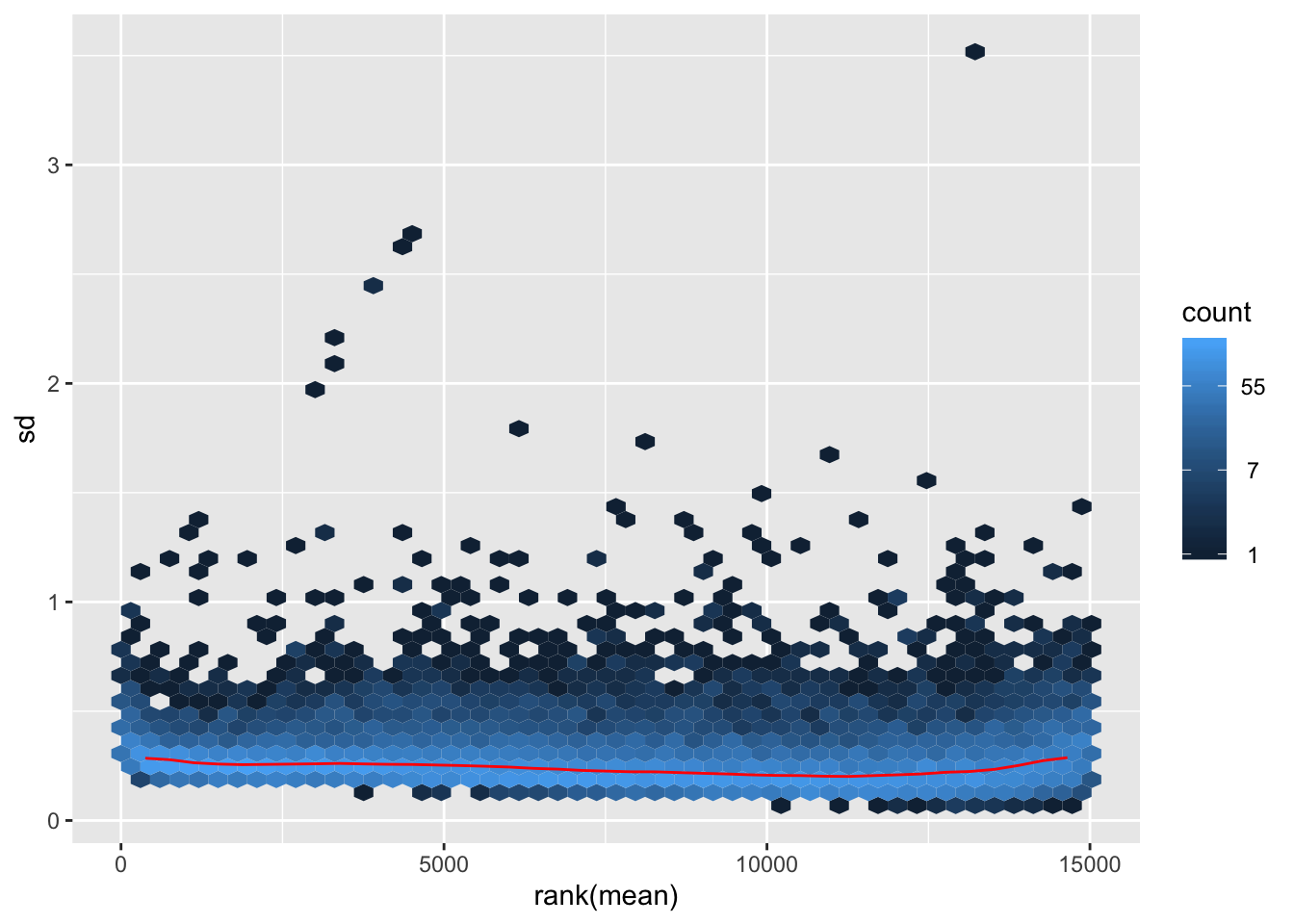
meanSdPlot(mat0)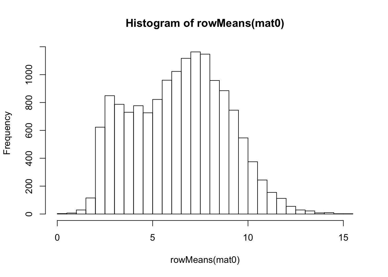
VST on original count data
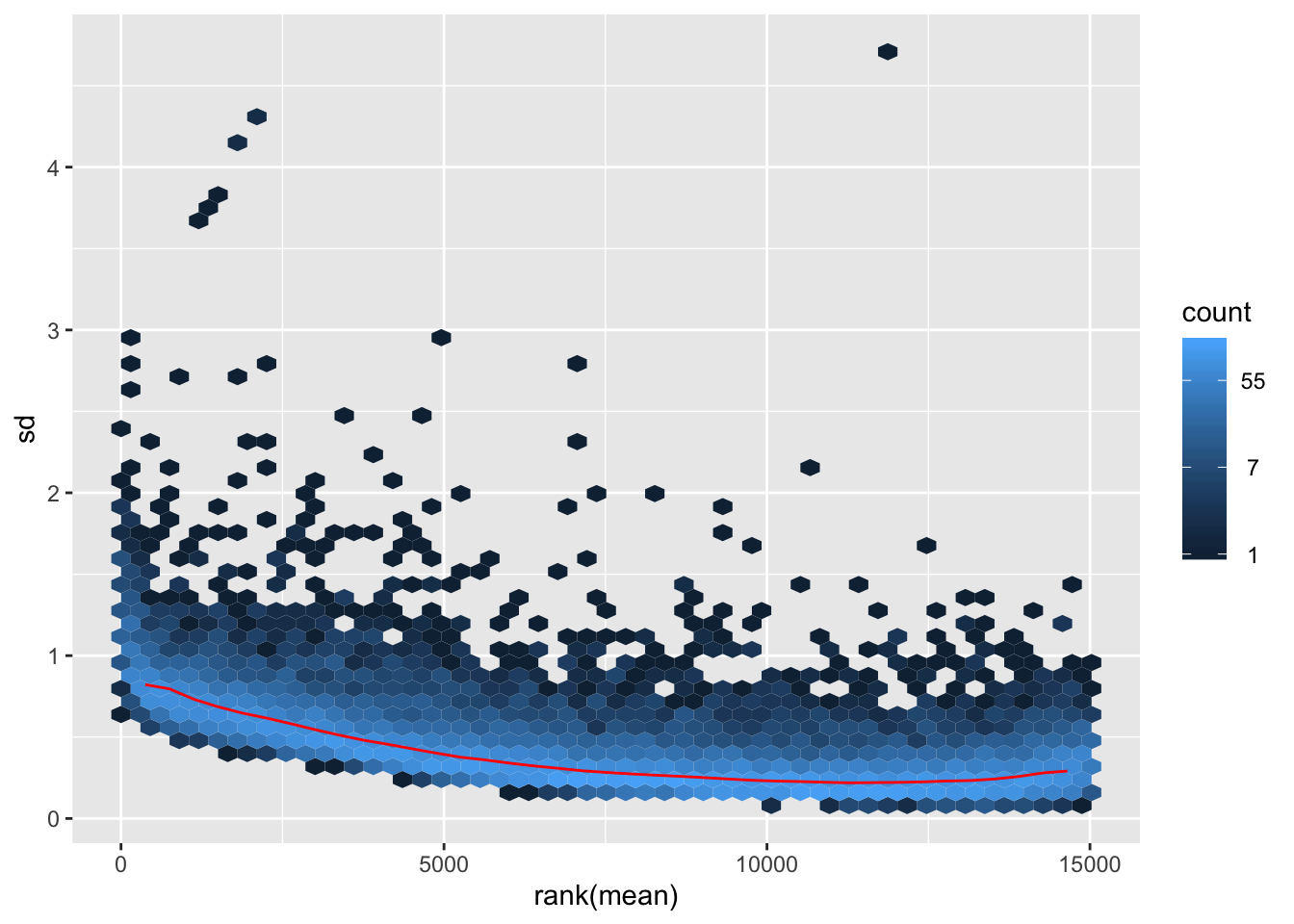
## vst
vsd <- vst(dds)
mat1 <- assay(vsd)
hist(rowMeans(mat1), breaks=50)
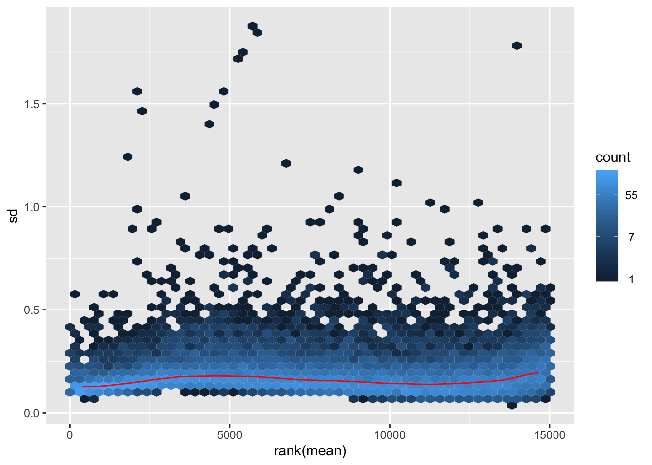
meanSdPlot(mat1)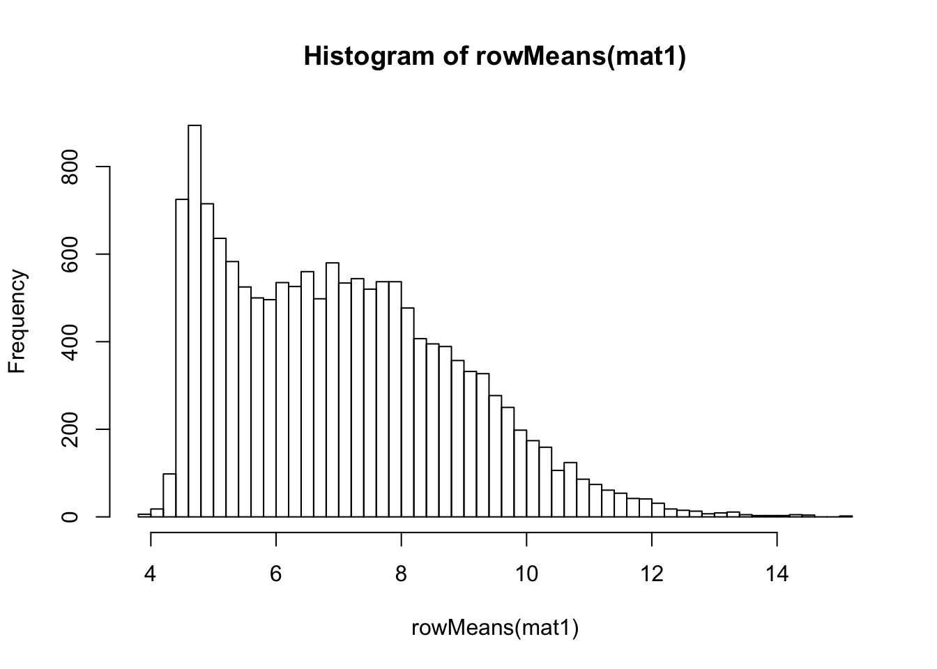
rlog-transformation on original count data
## rlog
rld <- rlog(dds)
## rlog() may take a long time with 50 or more samples,
## vst() is a much faster transformationmat2 <- assay(rld)
hist(rowMeans(mat2), breaks=50)
meanSdPlot(mat2)
Gene filtering
Working with the original data, we observe excessive low count genes. We will further filter the data by removing low count and low variance genes. First, let’s check the per gene mean and standard deviation.
## per gene mean count
gmeans <- rowMeans(mycount)
summary(gmeans)
## Min. 1st Qu. Median Mean 3rd Qu. Max.
## 1.17 24.20 104.67 385.77 329.92 39982.93## per gene standard deviation
gsd <- apply(mycount, 1, sd)
summary(gsd)## Min. 1st Qu. Median Mean 3rd Qu. Max.
## 2.73 14.45 53.76 207.71 168.46 21554.67Based on the above, it is reasonable to set the following thresholds for the mean and standard deviation.
## set thresholds
m.thred <- 10
sd.thred <- 5

## keep high count and high variation genes
ind.kp <- (gmeans > m.thred) & (gsd > sd.thred)

## filted count data
mycount.filt <- mycount[ind.kp,]
dim(mycount.filt)
## [1] 13169 75For data filtering, we remove the genes that have mean count below 10 and standard deviation below 5 across all samples. The filtered data has 13169 genes and 75 samples. Next, we build the DESeq2 data object for the filtered data.
## build dds object on the filtered count data
dds.filt <- DESeqDataSetFromMatrix(countData = mycount.filt,
                              colData = ctab,
                              design = ~ 1)
log2-transformation on filtered data
## log2-transformation
ntd.filt <- normTransform(dds.filt)
mat0.filt <- assay(ntd.filt)
hist(rowMeans(mat0.filt), breaks=50)
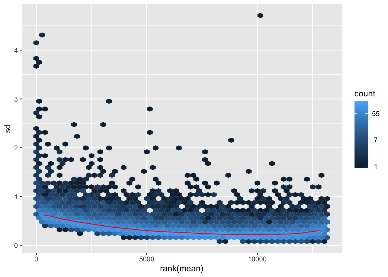
meanSdPlot(mat0.filt)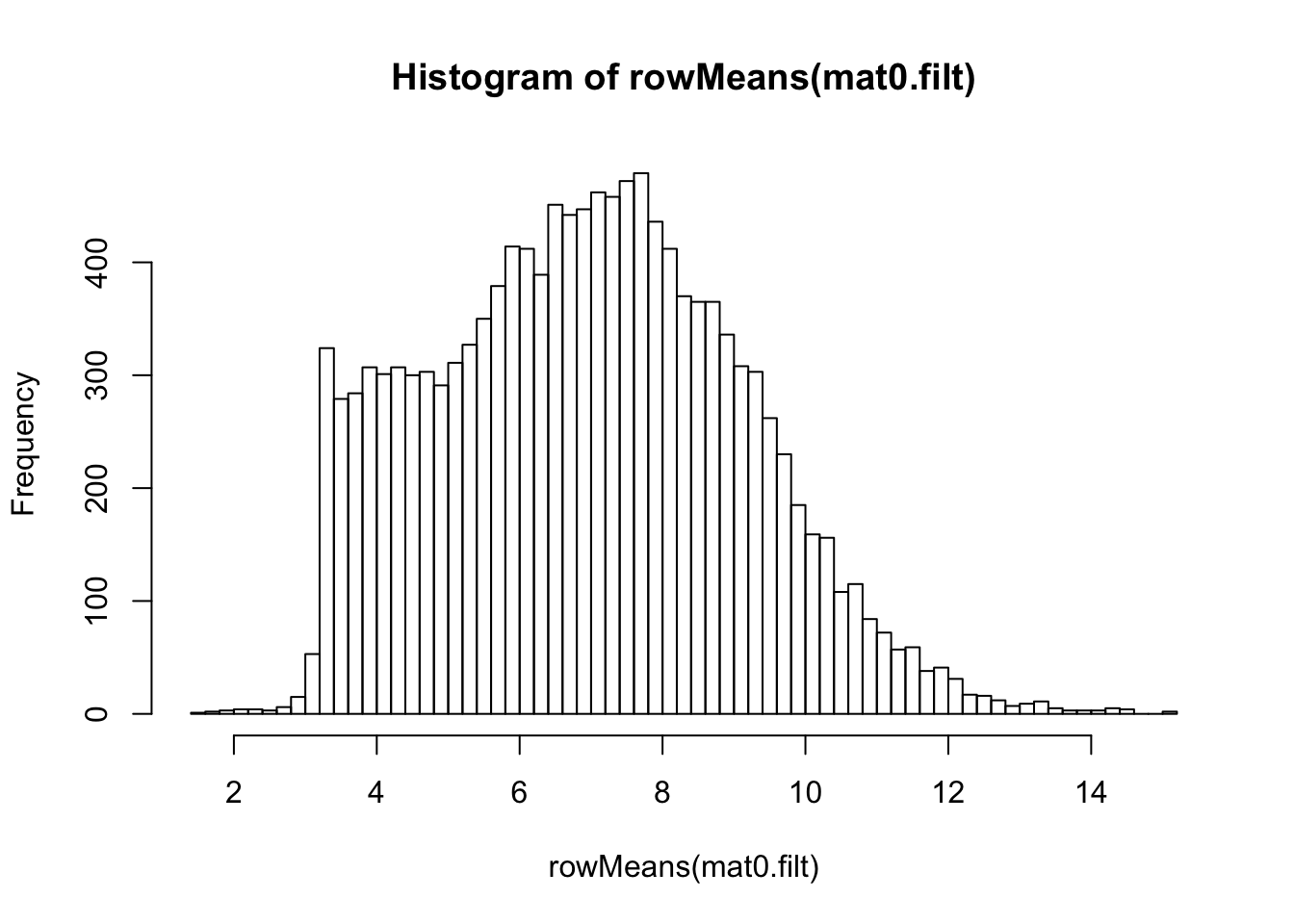
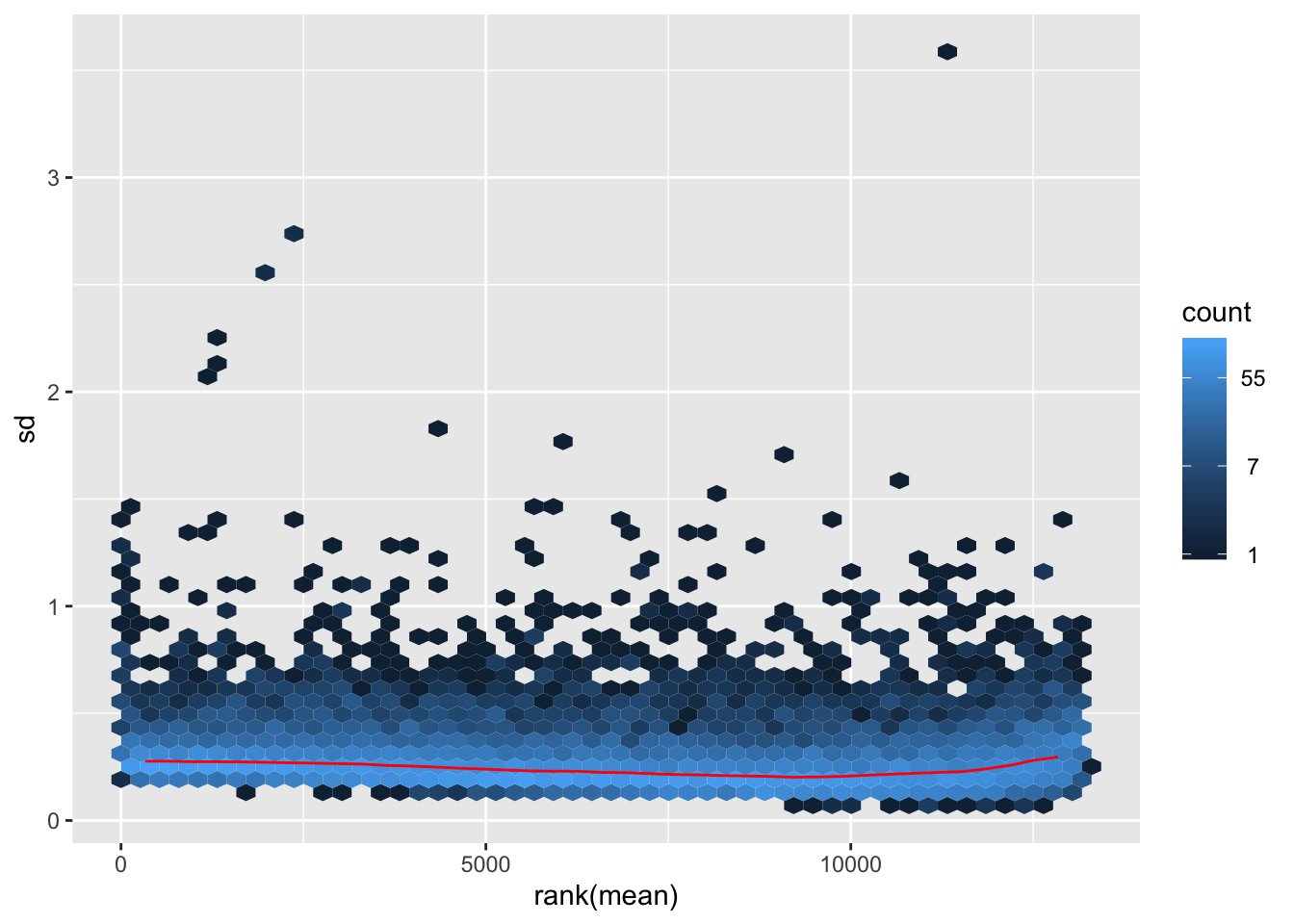
VST on filtered data
## vst
vsd.filt <- vst(dds.filt)
mat1.filt <- assay(vsd.filt)
hist(rowMeans(mat1.filt), breaks=50)
meanSdPlot(mat1.filt)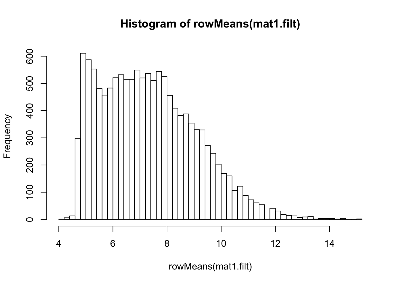
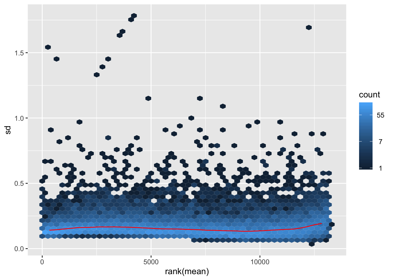
rlog-transformation on filtered data
## rlog
rld.filt <- rlog(dds.filt)
## rlog() may take a long time with 50 or more samples,
## vst() is a much faster transformationmat2.filt <- assay(rld.filt)
hist(rowMeans(mat2.filt), breaks=50)
meanSdPlot(mat2.filt)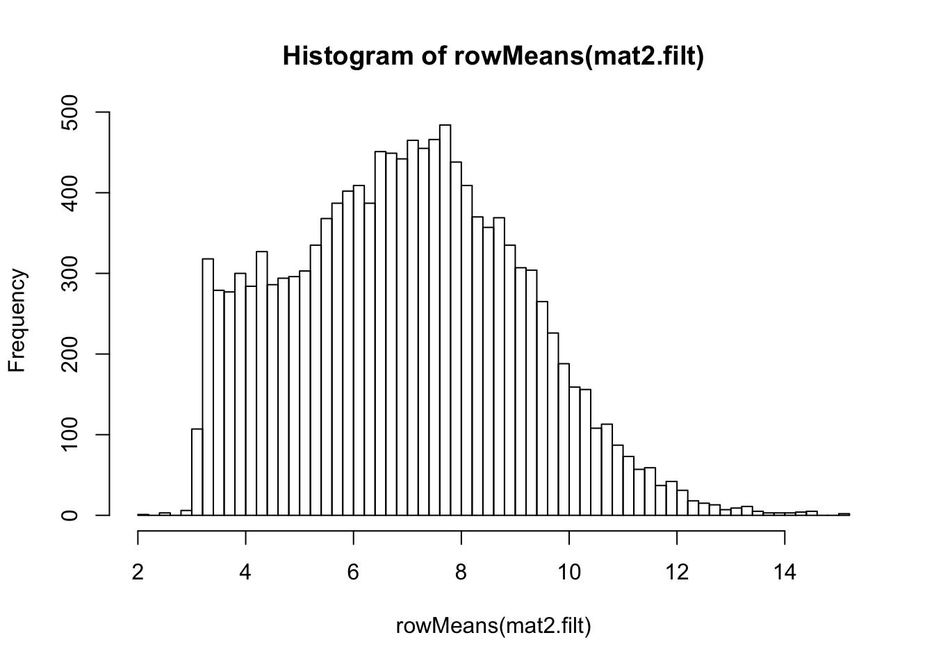
Final preprocessed data
We decide to use the rlog transformed data on the filtered data.
## rename
dat.filt10 <- mat2.filt
The original data use Ensembl gene ids, and we map them to gene symbols using EnsDb.Hsapiens.v86.
library(EnsDb.Hsapiens.v86)
mymap <- select(EnsDb.Hsapiens.v86, key=rownames(dat.filt10), columns=c("SYMBOL"), keytype="GENEID")
detach("package:EnsDb.Hsapiens.v86", unload=TRUE)
detach("package:ensembldb", unload=TRUE)
## the final data only keep the genes that have unique gene symbols
dat.filt10.symbol <- dat.filt10 %>% as_tibble(rownames = NA) %>% rownames_to_column() %>%
right_join(mymap %>% distinct(SYMBOL, .keep_all = TRUE), by = c("rowname"="GENEID")) %>%
dplyr::select(-rowname) %>% column_to_rownames(var = "SYMBOL") %>%
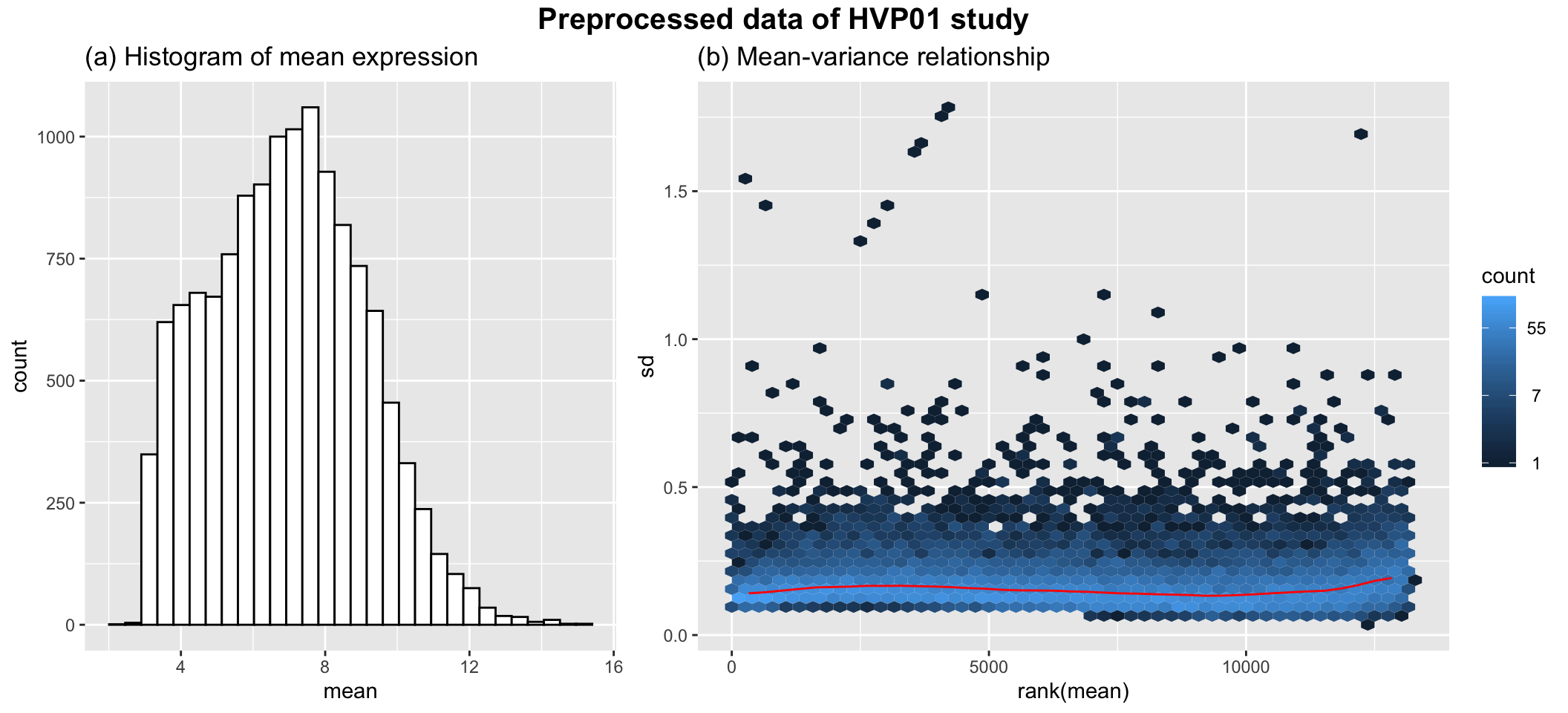
as.matrix()Finally, we are going to work with dat.filt10.symbol, which has 13157 genes and 75 samples. After the filtering and data transformation, the following figure shows that the final data follows a nice close-to-normal distribution, and the variance is stable across the range of mean expression.
## combined plot
g1 <- ggplot(data.frame("mean"=rowMeans(dat.filt10.symbol)), aes(x=mean)) +
  geom_histogram(color="black", fill="white") + ggtitle("(a) Histogram of mean expression")
g2 <- meanSdPlot(dat.filt10.symbol, plot = FALSE)$gg + ggtitle("(b) Mean-variance relationship")
g <- grid.arrange(g1, g2, nrow=1, widths = c(1, 1.5), top=textGrob("Preprocessed data of HVP01 study", gp = gpar(fontface = 2, fontsize = 15)))